Complete PySpark Learning Roadmap
Professional Guide with Practical Examples
Table of Contents
- Introduction to PySpark
- Environment Setup
- Core Concepts and Architecture
- RDD (Resilient Distributed Datasets)
- DataFrames and Datasets
- Spark SQL
- Data Transformations and Actions
- Performance Optimization
- Advanced Topics
- Real-World Projects
- Interview Questions and Answers
1. Introduction to PySpark
What is PySpark?
PySpark is the Python API for Apache Spark, a unified analytics engine for large-scale data processing. It enables parallel data processing across clusters, making it ideal for big data analytics.
Key Features
- Speed: 100x faster than Hadoop MapReduce for in-memory computations
- Ease of Use: High-level APIs in Python
- Unified Engine: Batch processing, streaming, machine learning, and graph processing
- Fault Tolerance: Automatic recovery from node failures
- Scalability: Process petabytes of data across thousands of nodes
When to Use PySpark
- Processing large datasets (GB to PB scale)
- ETL operations on big data
- Real-time streaming analytics
- Machine learning on distributed data
- Complex data transformations requiring parallel processing
2. Environment Setup
Installation Methods
Method 1: Local Installation
# Install Java (required)
# Download Java 8 or 11 from Oracle/OpenJDK

# Install PySpark using pip
pip install pyspark

# Verify installation
pyspark --version
Method 2: Databricks Community Edition (Recommended for Beginners)
- Go to databricks.com/try-databricks
- Sign up for Community Edition (free)
- Create a notebook and start coding
Method 3: Google Colab
# Install PySpark in Colab
!pip install pyspark

# Import and create SparkSession
from pyspark.sql import SparkSession
spark = SparkSession.builder.appName("MyApp").getOrCreate()
Setting Up Local Development Environment
# Create SparkSession - Entry point for PySpark
from pyspark.sql import SparkSession

spark = SparkSession.builder \
    .appName("Learning PySpark") \
    .master("local[*]") \
    .config("spark.driver.memory", "4g") \
    .getOrCreate()

# Verify setup
print(f"Spark Version: {spark.version}")
print(f"Application Name: {spark.sparkContext.appName}")
3. Core Concepts and Architecture
Spark Architecture Components
Master-Worker Architecture
- Driver: Runs the main() function, creates SparkContext
- Cluster Manager: Allocates resources (YARN, Mesos, Kubernetes, Standalone)
- Executors: Worker nodes that execute tasks and store data
- Tasks: Units of work sent to executors
Key Concepts
- SparkContext: Connection to Spark cluster (for RDDs)
- SparkSession: Unified entry point (for DataFrames and SQL)
- Transformations: Lazy operations that define computation
- Actions: Trigger actual execution and return results
- DAG (Directed Acyclic Graph): Execution plan created by Spark
Lazy Evaluation
# Transformations are lazy - no execution yet
df = spark.read.csv("data.csv")
filtered_df = df.filter(df['age'] > 25)
result_df = filtered_df.select("name", "age")

# Action triggers execution of all transformations
result_df.show()  # Only now the execution happens
4. RDD (Resilient Distributed Datasets)
What are RDDs?
RDDs are the fundamental data structure of Spark – immutable, distributed collections of objects that can be processed in parallel.
Creating RDDs
# Method 1: From Python collection
data = [1, 2, 3, 4, 5, 6, 7, 8, 9, 10]
rdd = spark.sparkContext.parallelize(data, numSlices=4)

# Method 2: From text file
text_rdd = spark.sparkContext.textFile("data.txt")

# Method 3: From existing RDD
squared_rdd = rdd.map(lambda x: x * x)
RDD Transformations (Lazy)
# map(): Apply function to each element
rdd = spark.sparkContext.parallelize([1, 2, 3, 4, 5])
squared = rdd.map(lambda x: x ** 2)
# Result: [1, 4, 9, 16, 25]

# filter(): Select elements matching condition
even_numbers = rdd.filter(lambda x: x % 2 == 0)
# Result: [2, 4]

# flatMap(): Map then flatten
words_rdd = spark.sparkContext.parallelize(["hello world", "spark python"])
words = words_rdd.flatMap(lambda line: line.split(" "))
# Result: ["hello", "world", "spark", "python"]

# distinct(): Remove duplicates
duplicates_rdd = spark.sparkContext.parallelize([1, 2, 2, 3, 3, 3])
unique = duplicates_rdd.distinct()
# Result: [1, 2, 3]

# union(): Combine two RDDs
rdd1 = spark.sparkContext.parallelize([1, 2, 3])
rdd2 = spark.sparkContext.parallelize([4, 5, 6])
combined = rdd1.union(rdd2)
# Result: [1, 2, 3, 4, 5, 6]

# intersection(): Common elements
rdd1 = spark.sparkContext.parallelize([1, 2, 3, 4])
rdd2 = spark.sparkContext.parallelize([3, 4, 5, 6])
common = rdd1.intersection(rdd2)
# Result: [3, 4]

# groupByKey(): Group values by key
pairs = spark.sparkContext.parallelize([("a", 1), ("b", 2), ("a", 3)])
grouped = pairs.groupByKey().mapValues(list)
# Result: [("a", [1, 3]), ("b", [2])]

# reduceByKey(): Aggregate values by key
pairs = spark.sparkContext.parallelize([("a", 1), ("b", 2), ("a", 3), ("b", 4)])
summed = pairs.reduceByKey(lambda x, y: x + y)
# Result: [("a", 4), ("b", 6)]

# sortByKey(): Sort by key
sorted_rdd = pairs.sortByKey()
RDD Actions (Eager – Trigger Execution)
# collect(): Return all elements to driver
result = rdd.collect()
print(result)  # [1, 2, 3, 4, 5]

# count(): Count elements
count = rdd.count()
print(count)  # 5

# take(n): Return first n elements
first_three = rdd.take(3)
print(first_three)  # [1, 2, 3]

# first(): Return first element
first_element = rdd.first()
print(first_element)  # 1

# reduce(): Aggregate all elements
sum_all = rdd.reduce(lambda x, y: x + y)
print(sum_all)  # 15

# countByKey(): Count occurrences of each key
pairs = spark.sparkContext.parallelize([("a", 1), ("b", 2), ("a", 3)])
counts = pairs.countByKey()
print(counts)  # defaultdict(<class 'int'>, {'a': 2, 'b': 1})

# saveAsTextFile(): Save to file
rdd.saveAsTextFile("output/rdd_data")
Practical RDD Example: Word Count
# Classic word count example
text = """
Apache Spark is a unified analytics engine for big data processing
Spark provides high level APIs in Java Scala Python and R
Spark also supports rich set of libraries
"""

# Create RDD
lines = spark.sparkContext.parallelize(text.split('\n'))

# Word count logic
word_counts = lines \
    .flatMap(lambda line: line.lower().split()) \
    .filter(lambda word: word.strip() != '') \
    .map(lambda word: (word, 1)) \
    .reduceByKey(lambda a, b: a + b) \
    .sortBy(lambda x: x[1], ascending=False)

# Display results
for word, count in word_counts.take(10):
    print(f"{word}: {count}")
5. DataFrames and Datasets
DataFrames Overview
DataFrames are distributed collections of data organized into named columns, similar to tables in relational databases or pandas DataFrames, but optimized for distributed processing.
Creating DataFrames
from pyspark.sql import Row
from pyspark.sql.types import StructType, StructField, StringType, IntegerType, DoubleType

# Method 1: From Python list
data = [
    ("John", 28, "Engineering", 75000),
    ("Jane", 32, "Marketing", 68000),
    ("Mike", 45, "Engineering", 95000),
    ("Sarah", 29, "HR", 62000),
    ("Tom", 38, "Marketing", 78000)
]

columns = ["name", "age", "department", "salary"]
df = spark.createDataFrame(data, columns)
df.show()

# Method 2: From dictionary
data_dict = [
    {"name": "John", "age": 28, "salary": 75000},
    {"name": "Jane", "age": 32, "salary": 68000}
]
df = spark.createDataFrame(data_dict)

# Method 3: With explicit schema
schema = StructType([
    StructField("name", StringType(), True),
    StructField("age", IntegerType(), True),
    StructField("department", StringType(), True),
    StructField("salary", DoubleType(), True)
])

df = spark.createDataFrame(data, schema)

# Method 4: From CSV file
df = spark.read.csv("employees.csv", header=True, inferSchema=True)

# Method 5: From JSON
df = spark.read.json("employees.json")

# Method 6: From Parquet (recommended for big data)
df = spark.read.parquet("employees.parquet")

# Method 7: From database
df = spark.read \
    .format("jdbc") \
    .option("url", "jdbc:postgresql://localhost:5432/mydb") \
    .option("dbtable", "employees") \
    .option("user", "username") \
    .option("password", "password") \
    .load()
Basic DataFrame Operations
# Display data
df.show()  # Show first 20 rows
df.show(5, truncate=False)  # Show 5 rows, no truncation

# Schema information
df.printSchema()
df.dtypes  # List of (column_name, type) tuples
df.columns  # List of column names

# Basic statistics
df.describe().show()
df.count()  # Number of rows
df.select("age").summary().show()

# Select columns
df.select("name", "age").show()
df.select(df.name, df.age).show()
df.select(df["name"], df["age"]).show()

# Select with expressions
from pyspark.sql.functions import col
df.select(col("name"), (col("salary") * 1.1).alias("new_salary")).show()

# Add new column
df = df.withColumn("bonus", col("salary") * 0.1)
df = df.withColumn("total_comp", col("salary") + col("bonus"))

# Rename column
df = df.withColumnRenamed("name", "employee_name")

# Drop column
df = df.drop("bonus")

# Filter rows
df.filter(df.age > 30).show()
df.filter((df.age > 30) & (df.salary > 70000)).show()
df.where(df.department == "Engineering").show()

# Sort
df.sort("age").show()
df.sort(col("age").desc()).show()
df.orderBy(col("salary").desc(), col("age").asc()).show()

# Limit
df.limit(5).show()

# Drop duplicates
df = df.dropDuplicates()
df = df.dropDuplicates(["department"])

# Handle null values
df = df.dropna()  # Drop rows with any null
df = df.dropna(subset=["age", "salary"])  # Drop if null in specific columns
df = df.fillna({"age": 0, "department": "Unknown"})  # Fill nulls
Aggregations and Grouping
from pyspark.sql import functions as F

# Group by and aggregate
df.groupBy("department").count().show()

df.groupBy("department").agg(
    F.avg("salary").alias("avg_salary"),
    F.max("salary").alias("max_salary"),
    F.min("salary").alias("min_salary"),
    F.sum("salary").alias("total_salary"),
    F.count("*").alias("employee_count")
).show()

# Multiple grouping columns
df.groupBy("department", "age").count().show()

# Aggregate without grouping
df.agg(
    F.avg("salary").alias("avg_salary"),
    F.stddev("salary").alias("std_salary")
).show()

# Window functions
from pyspark.sql.window import Window

# Rank employees by salary within department
window_spec = Window.partitionBy("department").orderBy(col("salary").desc())

df_ranked = df.withColumn("rank", F.rank().over(window_spec))
df_ranked.show()

# Running total
window_spec_running = Window.partitionBy("department").orderBy("age") \
    .rowsBetween(Window.unboundedPreceding, Window.currentRow)

df_running = df.withColumn(
    "running_total_salary",
    F.sum("salary").over(window_spec_running)
)
df_running.show()
Joins
# Create sample DataFrames
employees = spark.createDataFrame([
    (1, "John", "Engineering"),
    (2, "Jane", "Marketing"),
    (3, "Mike", "Engineering"),
    (4, "Sarah", "HR")
], ["emp_id", "name", "dept_name"])

departments = spark.createDataFrame([
    ("Engineering", "Building A"),
    ("Marketing", "Building B"),
    ("HR", "Building C"),
    ("Finance", "Building D")
], ["dept_name", "location"])

# Inner join (default)
result = employees.join(departments, "dept_name", "inner")
result.show()

# Left join
result = employees.join(departments, "dept_name", "left")
result.show()

# Right join
result = employees.join(departments, "dept_name", "right")
result.show()

# Full outer join
result = employees.join(departments, "dept_name", "outer")
result.show()

# Join on different column names
salaries = spark.createDataFrame([
    (1, 75000),
    (2, 68000),
    (3, 95000)
], ["employee_id", "salary"])

result = employees.join(
    salaries,
    employees.emp_id == salaries.employee_id,
    "inner"
).drop(salaries.employee_id)
result.show()

# Self join
result = employees.alias("e1").join(
    employees.alias("e2"),
    col("e1.dept_name") == col("e2.dept_name"),
    "inner"
).filter(col("e1.emp_id") < col("e2.emp_id"))
result.select("e1.name", "e2.name", "e1.dept_name").show()
6. Spark SQL
SQL Queries on DataFrames
# Register DataFrame as temporary view
df.createOrReplaceTempView("employees")

# Run SQL queries
result = spark.sql("""
    SELECT department,
           AVG(salary) as avg_salary,
           COUNT(*) as employee_count
    FROM employees
    GROUP BY department
    HAVING AVG(salary) > 70000
    ORDER BY avg_salary DESC
""")
result.show()

# Complex SQL example
spark.sql("""
    SELECT
        name,
        department,
        salary,
        RANK() OVER (PARTITION BY department ORDER BY salary DESC) as rank,
        CASE
            WHEN salary > 80000 THEN 'High'
            WHEN salary > 60000 THEN 'Medium'
            ELSE 'Low'
        END as salary_category
    FROM employees
""").show()

# Join using SQL
employees.createOrReplaceTempView("employees")
departments.createOrReplaceTempView("departments")

result = spark.sql("""
    SELECT e.name, e.dept_name, d.location
    FROM employees e
    LEFT JOIN departments d ON e.dept_name = d.dept_name
""")
result.show()

# Subqueries
spark.sql("""
    SELECT name, salary
    FROM employees
    WHERE salary > (SELECT AVG(salary) FROM employees)
""").show()

# Common Table Expressions (CTE)
spark.sql("""
    WITH dept_stats AS (
        SELECT department, AVG(salary) as avg_salary
        FROM employees
        GROUP BY department
    )
    SELECT e.name, e.salary, d.avg_salary
    FROM employees e
    JOIN dept_stats d ON e.department = d.department
    WHERE e.salary > d.avg_salary
""").show()
7. Data Transformations and Actions
Built-in Functions
from pyspark.sql import functions as F
from pyspark.sql.types import *

# String functions
df = df.withColumn("name_upper", F.upper(col("name")))
df = df.withColumn("name_lower", F.lower(col("name")))
df = df.withColumn("name_length", F.length(col("name")))
df = df.withColumn("name_substring", F.substring(col("name"), 1, 3))
df = df.withColumn("name_concat", F.concat(col("name"), F.lit(" - "), col("department")))
df = df.withColumn("name_trimmed", F.trim(col("name")))

# Numeric functions
df = df.withColumn("salary_rounded", F.round(col("salary"), -3))
df = df.withColumn("salary_ceil", F.ceil(col("salary") / 1000))
df = df.withColumn("salary_floor", F.floor(col("salary") / 1000))
df = df.withColumn("abs_diff", F.abs(col("salary") - 70000))

# Date functions
from datetime import datetime, date

df_dates = spark.createDataFrame([
    (1, datetime(2024, 1, 15)),
    (2, datetime(2024, 6, 20)),
    (3, datetime(2023, 12, 10))
], ["id", "join_date"])

df_dates = df_dates.withColumn("year", F.year(col("join_date")))
df_dates = df_dates.withColumn("month", F.month(col("join_date")))
df_dates = df_dates.withColumn("day", F.dayofmonth(col("join_date")))
df_dates = df_dates.withColumn("days_since_join", F.datediff(F.current_date(), col("join_date")))
df_dates = df_dates.withColumn("next_year", F.add_months(col("join_date"), 12))
df_dates.show()

# Conditional functions
df = df.withColumn(
    "salary_grade",
    F.when(col("salary") > 80000, "A")
     .when(col("salary") > 60000, "B")
     .otherwise("C")
)

# Null handling
df = df.withColumn("salary_filled", F.coalesce(col("salary"), F.lit(50000)))
df = df.withColumn("is_null", F.isnull(col("salary")))
df = df.withColumn("is_not_null", F.col("salary").isNotNull())

# Array functions
df_arrays = spark.createDataFrame([
    (1, ["Python", "Scala", "Java"]),
    (2, ["R", "Python"]),
    (3, ["Java"])
], ["id", "skills"])

df_arrays = df_arrays.withColumn("num_skills", F.size(col("skills")))
df_arrays = df_arrays.withColumn("has_python", F.array_contains(col("skills"), "Python"))
df_arrays = df_arrays.withColumn("first_skill", F.element_at(col("skills"), 1))
df_arrays.show(truncate=False)

# Explode arrays
df_exploded = df_arrays.select("id", F.explode(col("skills")).alias("skill"))
df_exploded.show()

# JSON parsing
json_data = spark.createDataFrame([
    (1, '{"name": "John", "age": 30}'),
    (2, '{"name": "Jane", "age": 25}')
], ["id", "json_str"])

from pyspark.sql.functions import from_json

json_schema = StructType([
    StructField("name", StringType()),
    StructField("age", IntegerType())
])

json_data = json_data.withColumn("parsed", from_json(col("json_str"), json_schema))
json_data = json_data.select("id", "parsed.*")
json_data.show()
User Defined Functions (UDFs)
from pyspark.sql.functions import udf
from pyspark.sql.types import StringType, IntegerType

# Simple UDF
def categorize_age(age):
    if age < 30:
        return "Young"
    elif age < 50:
        return "Middle-aged"
    else:
        return "Senior"

categorize_age_udf = udf(categorize_age, StringType())
df = df.withColumn("age_category", categorize_age_udf(col("age")))

# UDF with decorator
@udf(returnType=IntegerType())
def calculate_bonus(salary):
    if salary > 80000:
        return int(salary * 0.15)
    else:
        return int(salary * 0.10)

df = df.withColumn("bonus", calculate_bonus(col("salary")))

# Pandas UDF (vectorized, much faster)
from pyspark.sql.functions import pandas_udf
import pandas as pd

@pandas_udf(IntegerType())
def calculate_bonus_pandas(salary: pd.Series) -> pd.Series:
    return (salary * 0.10).astype(int)

df = df.withColumn("bonus_pandas", calculate_bonus_pandas(col("salary")))
Practical Example: Complete ETL Pipeline
# Step 1: Read data from multiple sources
sales_df = spark.read.csv("sales_data.csv", header=True, inferSchema=True)
customers_df = spark.read.json("customers.json")
products_df = spark.read.parquet("products.parquet")

# Step 2: Data cleaning
# Remove duplicates
sales_df = sales_df.dropDuplicates(["transaction_id"])

# Handle nulls
sales_df = sales_df.fillna({
    "quantity": 0,
    "discount": 0.0
})

# Filter invalid data
sales_df = sales_df.filter(
    (col("quantity") > 0) &
    (col("price") > 0) &
    (col("transaction_date").isNotNull())
)

# Step 3: Data transformation
# Add calculated columns
sales_df = sales_df.withColumn(
    "total_amount",
    col("quantity") * col("price") * (1 - col("discount"))
)

sales_df = sales_df.withColumn(
    "transaction_year",
    F.year(col("transaction_date"))
)

sales_df = sales_df.withColumn(
    "transaction_month",
    F.month(col("transaction_date"))
)

# Step 4: Join datasets
result_df = sales_df \
    .join(customers_df, "customer_id", "left") \
    .join(products_df, "product_id", "left")

# Step 5: Aggregation and analytics
monthly_sales = result_df.groupBy(
    "transaction_year",
    "transaction_month",
    "product_category"
).agg(
    F.sum("total_amount").alias("total_revenue"),
    F.count("transaction_id").alias("transaction_count"),
    F.avg("total_amount").alias("avg_transaction_value"),
    F.countDistinct("customer_id").alias("unique_customers")
)

# Step 6: Window functions for ranking
window_spec = Window.partitionBy("transaction_year", "transaction_month") \
    .orderBy(col("total_revenue").desc())

monthly_sales = monthly_sales.withColumn(
    "category_rank",
    F.rank().over(window_spec)
)

# Step 7: Filter top performers
top_categories = monthly_sales.filter(col("category_rank") <= 5)

# Step 8: Write results
top_categories.write \
    .mode("overwrite") \
    .partitionBy("transaction_year", "transaction_month") \
    .parquet("output/top_categories")

# Also write to CSV for reporting
top_categories.coalesce(1).write \
    .mode("overwrite") \
    .option("header", "true") \
    .csv("output/top_categories_report")
8. Performance Optimization
Caching and Persistence
# Cache in memory (default storage level)
df.cache()
df.count()  # First action triggers caching
df.show()   # Second action uses cached data

# Unpersist when done
df.unpersist()

# Different storage levels
from pyspark import StorageLevel

df.persist(StorageLevel.MEMORY_AND_DISK)  # Spill to disk if memory full
df.persist(StorageLevel.DISK_ONLY)  # Store only on disk
df.persist(StorageLevel.MEMORY_ONLY_2)  # Replicate cached data

# Check if cached
print(df.is_cached)
Partitioning
# Check current partitions
print(f"Number of partitions: {df.rdd.getNumPartitions()}")

# Repartition (shuffle data)
df_repartitioned = df.repartition(10)
df_repartitioned = df.repartition(10, "department")  # Partition by column

# Coalesce (reduce partitions without shuffle - more efficient)
df_coalesced = df.coalesce(5)

# Partition data when writing
df.write \
    .partitionBy("year", "month") \
    .parquet("output/partitioned_data")

# Read specific partitions
df_filtered = spark.read \
    .parquet("output/partitioned_data") \
    .filter((col("year") == 2024) & (col("month") == 1))
Broadcast Joins
from pyspark.sql.functions import broadcast

# Small dimension table
departments_df = spark.read.csv("departments.csv", header=True)

# Large fact table
employees_df = spark.read.csv("employees.csv", header=True)

# Broadcast small table to all executors
result = employees_df.join(
    broadcast(departments_df),
    "department_id"
)

# Automatic broadcast (configure threshold)
spark.conf.set("spark.sql.autoBroadcastJoinThreshold", 10485760)  # 10MB
Optimizing Transformations
# Bad: Multiple passes over data
df_filtered = df.filter(col("age") > 30)
df_selected = df_filtered.select("name", "salary")
df_sorted = df_selected.sort("salary")

# Good: Chain operations
df_optimized = df \
    .filter(col("age") > 30) \
    .select("name", "salary") \
    .sort("salary")

# Bad: Using UDFs when built-in functions exist
@udf(StringType())
def upper_case(s):
    return s.upper()

df = df.withColumn("name_upper", upper_case(col("name")))

# Good: Use built-in functions
df = df.withColumn("name_upper", F.upper(col("name")))

# Avoid collect() on large datasets
# Bad
all_data = df.collect()  # Brings all data to driver

# Good: Use limit or aggregations
sample_data = df.limit(100).collect()
summary = df.groupBy("department").count().collect()
Configuration Tuning
# Memory configuration
spark = SparkSession.builder \
    .config("spark.driver.memory", "8g") \
    .config("spark.executor.memory", "16g") \
    .config("spark.executor.cores", "4") \
    .config("spark.executor.instances", "10") \
    .getOrCreate()

# Shuffle optimization
spark.conf.set("spark.sql.shuffle.partitions", "200")  # Default is 200
spark.conf.set("spark.sql.adaptive.enabled", "true")  # Enable AQE
spark.conf.set("spark.sql.adaptive.coalescePartitions.enabled", "true")

# Serialization
spark.conf.set("spark.serializer", "org.apache.spark.serializer.KryoSerializer")

# Dynamic allocation
spark.conf.set("spark.dynamicAllocation.enabled", "true")
spark.conf.set("spark.dynamicAllocation.minExecutors", "2")
spark.conf.set("spark.dynamicAllocation.maxExecutors", "20")
Best Practices Checklist
- Use DataFrames over RDDs for better optimization
- Cache wisely – only cache DataFrames used multiple times
- Partition appropriately – balance parallelism with overhead
- Use built-in functions instead of UDFs when possible
- Broadcast small tables in joins
- Avoid wide transformations when possible
- Filter early to reduce data volume
- Use columnar formats (Parquet, ORC) for storage
- Enable Adaptive Query Execution (AQE) in Spark 3.x
- Monitor and profile your jobs using Spark UI
9. Advanced Topics
Structured Streaming
from pyspark.sql.functions import window, col

# Read streaming data
streaming_df = spark.readStream \
    .format("kafka") \
    .option("kafka.bootstrap.servers", "localhost:9092") \
    .option("subscribe", "transactions") \
    .load()

# Parse JSON from Kafka
from pyspark.sql.functions import from_json

schema = StructType([
    StructField("transaction_id", StringType()),
    StructField("amount", DoubleType()),
    StructField("timestamp", TimestampType())
])

parsed_df = streaming_df.select(
    from_json(col("value").cast("string"), schema).alias("data")
).select("data.*")

# Window aggregation
windowed_counts = parsed_df \
    .withWatermark("timestamp", "10 minutes") \
    .groupBy(
        window(col("timestamp"), "5 minutes", "1 minute")
    ).agg(
        F.sum("amount").alias("total_amount"),
        F.count("*").alias("transaction_count")
    )

# Write streaming output
query = windowed_counts.writeStream \
    .outputMode("update") \
    .format("console") \
    .trigger(processingTime="30 seconds") \
    .start()

# File source streaming
file_stream = spark.readStream \
    .format("csv") \
    .option("header", "true") \
    .schema(schema) \
    .load("input_directory/")

# Write to Parquet with checkpointing
file_stream.writeStream \
    .format("parquet") \
    .option("path", "output/") \
    .option("checkpointLocation", "checkpoint/") \
    .start()
Machine Learning with MLlib
from pyspark.ml.feature import VectorAssembler, StandardScaler
from pyspark.ml.regression import LinearRegression
from pyspark.ml.classification import LogisticRegression, RandomForestClassifier
from pyspark.ml.evaluation import RegressionEvaluator, BinaryClassificationEvaluator
from pyspark.ml import Pipeline

# Prepare data
data = spark.read.csv("training_data.csv", header=True, inferSchema=True)

# Feature engineering
assembler = VectorAssembler(
    inputCols=["feature1", "feature2", "feature3"],
    outputCol="features"
)

scaler = StandardScaler(
    inputCol="features",
    outputCol="scaled_features"
)

# Create model
lr = LinearRegression(
    featuresCol="scaled_features",
    labelCol="target",
    maxIter=100,
    regParam=0.1
)

# Create pipeline
pipeline = Pipeline(stages=[assembler, scaler, lr])

# Split data
train_data, test_data = data.randomSplit([0.8, 0.2], seed=42)

# Train model
model = pipeline.fit(train_data)

# Make predictions
predictions = model.transform(test_data)

# Evaluate
evaluator = RegressionEvaluator(
    labelCol="target",
    predictionCol="prediction",
    metricName="rmse"
)
rmse = evaluator.evaluate(predictions)
print(f"RMSE: {rmse}")

# Classification example
rf = RandomForestClassifier(
    featuresCol="scaled_features",
    labelCol="label",
    numTrees=100
)

rf_pipeline = Pipeline(stages=[assembler, scaler, rf])
rf_model = rf_pipeline.fit(train_data)

# Evaluate classification
rf_predictions = rf_model.transform(test_data)
evaluator = BinaryClassificationEvaluator(labelCol="label")
auc = evaluator.evaluate(rf_predictions)
print(f"AUC: {auc}")
Graph Processing with GraphFrames
# Install: pip install graphframes

from graphframes import GraphFrame

# Create vertices DataFrame
vertices = spark.createDataFrame([
    ("1", "Alice", 34),
    ("2", "Bob", 36),
    ("3", "Charlie", 30),
    ("4", "David", 29)
], ["id", "name", "age"])

# Create edges DataFrame
edges = spark.createDataFrame([
    ("1", "2", "friend"),
    ("2", "3", "follow"),
    ("3", "4", "friend"),
    ("1", "4", "follow")
], ["src", "dst", "relationship"])

# Create graph
graph = GraphFrame(vertices, edges)

# Query
graph.vertices.show()
graph.edges.show()

# Find motifs
motifs = graph.find("(a)-[e]->(b); (b)-[e2]->(c)")
motifs.show()

# PageRank
results = graph.pageRank(resetProbability=0.15, maxIter=10)
results.vertices.select("id", "name", "pagerank").show()

# Connected components
components = graph.connectedComponents()
components.show()

# Shortest paths
paths = graph.shortestPaths(landmarks=["1", "4"])
paths.show()
10. Real-World Projects
Project 1: E-Commerce Sales Analysis
# Objective: Analyze sales patterns and customer behavior

# Step 1: Load data
orders = spark.read.csv("orders.csv", header=True, inferSchema=True)
customers = spark.read.csv("customers.csv", header=True, inferSchema=True)
products = spark.read.csv("products.csv", header=True, inferSchema=True)

# Step 2: Data preparation
orders = orders.withColumn("order_date", F.to_date(col("order_date")))
orders = orders.withColumn("order_year", F.year(col("order_date")))
orders = orders.withColumn("order_month", F.month(col("order_date")))

# Step 3: Customer segmentation by purchase frequency
customer_orders = orders.groupBy("customer_id").agg(
    F.count("order_id").alias("order_count"),
    F.sum("total_amount").alias("total_spent"),
    F.avg("total_amount").alias("avg_order_value"),
    F.max("order_date").alias("last_order_date")
)

customer_orders = customer_orders.withColumn(
    "days_since_last_order",
    F.datediff(F.current_date(), col("last_order_date"))
)

customer_orders = customer_orders.withColumn(
    "customer_segment",
    F.when(col("order_count") >= 10, "VIP")
     .when(col("order_count") >= 5, "Regular")
     .otherwise("Occasional")
)

# Step 4: Product performance analysis
product_sales = orders.join(products, "product_id") \
    .groupBy("category", "product_name") \
    .agg(
        F.sum("quantity").alias("units_sold"),
        F.sum("total_amount").alias("revenue")
    )

window_spec = Window.partitionBy("category").orderBy(col("revenue").desc())
product_sales = product_sales.withColumn("rank", F.rank().over(window_spec))

top_products = product_sales.filter(col("rank") <= 5)

# Step 5: Monthly trends
monthly_trends = orders.groupBy("order_year", "order_month").agg(
    F.sum("total_amount").alias("monthly_revenue"),
    F.count("order_id").alias("monthly_orders"),
    F.countDistinct("customer_id").alias("unique_customers")
)

# Step 6: Cohort analysis
first_purchase = orders.groupBy("customer_id").agg(
    F.min("order_date").alias("first_purchase_date")
)

orders_with_cohort = orders.join(first_purchase, "customer_id")
orders_with_cohort = orders_with_cohort.withColumn(
    "cohort_month",
    F.date_format(col("first_purchase_date"), "yyyy-MM")
)

orders_with_cohort = orders_with_cohort.withColumn(
    "order_month",
    F.date_format(col("order_date"), "yyyy-MM")
)

cohort_analysis = orders_with_cohort.groupBy("cohort_month", "order_month") \
    .agg(F.countDistinct("customer_id").alias("customers"))

# Step 7: Save results
top_products.write.mode("overwrite").parquet("output/top_products")
customer_orders.write.mode("overwrite").parquet("output/customer_segments")
monthly_trends.write.mode("overwrite").parquet("output/monthly_trends")
Project 2: Log Analysis and Anomaly Detection
# Objective: Process server logs and detect anomalies

# Step 1: Parse log files
log_df = spark.read.text("server_logs/*.log")

# Extract information using regex
from pyspark.sql.functions import regexp_extract

log_pattern = r'^(\S+) - - \[([^\]]+)\] "([A-Z]+) ([^\s]+) HTTP/\d\.\d" (\d{3}) (\d+)'

parsed_logs = log_df.select(
    regexp_extract(col("value"), log_pattern, 1).alias("ip"),
    regexp_extract(col("value"), log_pattern, 2).alias("timestamp"),
    regexp_extract(col("value"), log_pattern, 3).alias("method"),
    regexp_extract(col("value"), log_pattern, 4).alias("endpoint"),
    regexp_extract(col("value"), log_pattern, 5).alias("status_code"),
    regexp_extract(col("value"), log_pattern, 6).alias("response_size")
)

# Convert data types
parsed_logs = parsed_logs \
    .withColumn("status_code", col("status_code").cast("int")) \
    .withColumn("response_size", col("response_size").cast("int")) \
    .withColumn("timestamp", F.to_timestamp(col("timestamp"), "dd/MMM/yyyy:HH:mm:ss Z"))

# Step 2: Calculate request rate per IP
window_5min = window(col("timestamp"), "5 minutes")

request_rates = parsed_logs.groupBy("ip", window_5min).agg(
    F.count("*").alias("request_count"),
    F.countDistinct("endpoint").alias("unique_endpoints")
)

# Step 3: Identify anomalies (potential DDoS)
stats = request_rates.select(
    F.mean("request_count").alias("mean_requests"),
    F.stddev("request_count").alias("stddev_requests")
).collect()[0]

mean_req = stats["mean_requests"]
stddev_req = stats["stddev_requests"]

anomalies = request_rates.filter(
    col("request_count") > (mean_req + 3 * stddev_req)
)

# Step 4: Error analysis
error_logs = parsed_logs.filter(col("status_code") >= 400)

error_summary = error_logs.groupBy("status_code", "endpoint").agg(
    F.count("*").alias("error_count")
).orderBy(col("error_count").desc())

# Step 5: Response time analysis (if available)
# Assuming we add response time to logs
slow_requests = parsed_logs.filter(col("response_size") > 1000000)  # > 1MB

endpoint_performance = parsed_logs.groupBy("endpoint").agg(
    F.avg("response_size").alias("avg_response_size"),
    F.max("response_size").alias("max_response_size"),
    F.count("*").alias("request_count")
)

# Step 6: Geographic analysis (using IP geolocation)
# Assume we have a geolocation lookup table
geo_lookup = spark.read.csv("geo_lookup.csv", header=True)

geo_analysis = parsed_logs.join(
    broadcast(geo_lookup),
    parsed_logs.ip == geo_lookup.ip_address,
    "left"
).groupBy("country", "city").agg(
    F.count("*").alias("requests"),
    F.countDistinct("ip").alias("unique_ips")
)

# Step 7: Save results
anomalies.write.mode("overwrite").parquet("output/anomalies")
error_summary.write.mode("overwrite").parquet("output/errors")
geo_analysis.write.mode("overwrite").parquet("output/geo_analysis")
Project 3: Real-Time Sensor Data Processing
# Objective: Process IoT sensor data in real-time

# Step 1: Define schema
sensor_schema = StructType([
    StructField("sensor_id", StringType()),
    StructField("timestamp", TimestampType()),
    StructField("temperature", DoubleType()),
    StructField("humidity", DoubleType()),
    StructField("pressure", DoubleType())
])

# Step 2: Read streaming data
sensor_stream = spark.readStream \
    .format("kafka") \
    .option("kafka.bootstrap.servers", "localhost:9092") \
    .option("subscribe", "sensor-data") \
    .option("startingOffsets", "latest") \
    .load()

# Step 3: Parse and clean data
parsed_stream = sensor_stream.select(
    from_json(col("value").cast("string"), sensor_schema).alias("data")
).select("data.*")

# Remove outliers
cleaned_stream = parsed_stream.filter(
    (col("temperature").between(-50, 100)) &
    (col("humidity").between(0, 100)) &
    (col("pressure").between(900, 1100))
)

# Step 4: Calculate rolling averages
windowed_avg = cleaned_stream \
    .withWatermark("timestamp", "10 minutes") \
    .groupBy(
        col("sensor_id"),
        window(col("timestamp"), "5 minutes", "1 minute")
    ).agg(
        F.avg("temperature").alias("avg_temp"),
        F.avg("humidity").alias("avg_humidity"),
        F.avg("pressure").alias("avg_pressure"),
        F.stddev("temperature").alias("stddev_temp")
    )

# Step 5: Detect anomalies
anomalies = windowed_avg.filter(
    (col("stddev_temp") > 5) |  # High temperature variance
    (col("avg_temp") > 35) |     # High average temperature
    (col("avg_humidity") > 90)   # High humidity
)

# Step 6: Alert generation
alerts = anomalies.select(
    col("sensor_id"),
    col("window.start").alias("alert_time"),
    F.lit("ANOMALY_DETECTED").alias("alert_type"),
    F.concat_ws(", ",
        F.when(col("avg_temp") > 35, "High Temperature"),
        F.when(col("avg_humidity") > 90, "High Humidity"),
        F.when(col("stddev_temp") > 5, "Temperature Fluctuation")
    ).alias("alert_reason")
)

# Step 7: Write to multiple sinks
# Console for monitoring
query1 = windowed_avg.writeStream \
    .outputMode("update") \
    .format("console") \
    .trigger(processingTime="30 seconds") \
    .start()

# Kafka for alerts
query2 = alerts.selectExpr("sensor_id as key", "to_json(struct(*)) as value") \
    .writeStream \
    .format("kafka") \
    .option("kafka.bootstrap.servers", "localhost:9092") \
    .option("topic", "sensor-alerts") \
    .option("checkpointLocation", "checkpoint/alerts") \
    .start()

# Parquet for historical analysis
query3 = cleaned_stream.writeStream \
    .format("parquet") \
    .option("path", "output/sensor_history") \
    .option("checkpointLocation", "checkpoint/history") \
    .partitionBy("sensor_id") \
    .trigger(processingTime="5 minutes") \
    .start()

# Wait for termination
spark.streams.awaitAnyTermination()
11. Interview Questions and Answers
Conceptual Questions
Q1: What is PySpark and how does it differ from Pandas?
A: PySpark is the Python API for Apache Spark, designed for distributed data processing across clusters. Key differences:
- Scale: PySpark handles TB-PB of data; Pandas works on single machine memory
- Processing: PySpark uses lazy evaluation and distributed computing; Pandas is eager and single-threaded
- Speed: PySpark is faster for large datasets due to parallelization
- Use Case: PySpark for big data ETL, ML at scale; Pandas for exploratory analysis on smaller datasets
Q2: Explain lazy evaluation in Spark.
A: Lazy evaluation means Spark doesn’t execute transformations immediately. Instead:
- Transformations build a DAG (Directed Acyclic Graph) of operations
- Execution only happens when an action is called
- Spark optimizes the entire execution plan before running
- Benefits: Optimized execution, reduced memory usage, fault tolerance
Example:
df = spark.read.csv("data.csv")  # Not executed
filtered = df.filter(col("age") > 25)  # Not executed
result = filtered.select("name")  # Not executed
result.show()  # NOW everything executes
Q3: What are transformations vs actions?
A:
- Transformations: Lazy operations that return new RDD/DataFrame (map, filter, join, groupBy)
- Actions: Trigger execution and return results to driver (collect, count, show, save)
Q4: Explain partitioning in Spark.
A: Partitioning splits data into chunks processed in parallel across executors:
- Default: Based on data size and cluster config
- Custom: Use
repartition()orpartitionBy() - Benefits: Parallelism, data locality, optimized shuffles
- Trade-off: Too few = underutilized resources; too many = overhead
Q5: What is the Catalyst Optimizer?
A: Catalyst is Spark SQL’s query optimizer that:
- Parses SQL/DataFrame operations into logical plan
- Applies optimization rules (predicate pushdown, column pruning)
- Generates physical execution plan
- Uses cost-based optimization to choose best strategy
Q6: Difference between cache() and persist()?
A:
cache(): Shorthand forpersist(MEMORY_ONLY)persist(): Allows specifying storage level (MEMORY_ONLY, MEMORY_AND_DISK, DISK_ONLY, etc.)- Both store computed DataFrame for reuse
- Use when DataFrame accessed multiple times
Q7: What is a broadcast join?
A: Broadcast join sends small table to all executors to avoid shuffle:
result = large_df.join(broadcast(small_df), "key")- Best for: Small dimension tables (<10MB default)
- Benefits: No shuffle, faster execution
- Alternative: Spark auto-broadcasts based on
spark.sql.autoBroadcastJoinThreshold
Q8: Explain shuffle in Spark.
A: Shuffle redistributes data across partitions:
- Triggered by: groupBy, join, repartition, distinct
- Process: Write to disk, transfer over network, read on other nodes
- Expensive: Disk I/O, network transfer, serialization
- Optimization: Minimize shuffles, use broadcast joins, tune partition count
Q9: What is a DAG in Spark?
A: DAG (Directed Acyclic Graph) represents execution plan:
- Nodes: RDD/DataFrame operations
- Edges: Dependencies between operations
- Stages: Groups of transformations without shuffle
- Benefits: Fault tolerance, optimization, parallel execution
Q10: Difference between RDD and DataFrame?
A:
- RDD: Low-level, unstructured, functional API, no optimization
- DataFrame: High-level, structured schema, SQL-like API, Catalyst optimization
- When to use: DataFrames for most cases; RDDs for unstructured data or custom partitioning
Coding Questions
Q11: Find the top 5 products by sales in each category.
from pyspark.sql.window import Window

window_spec = Window.partitionBy("category").orderBy(col("sales").desc())

result = df.withColumn("rank", F.rank().over(window_spec)) \
    .filter(col("rank") <= 5) \
    .select("category", "product", "sales", "rank")

result.show()
Q12: Calculate running total of sales by date.
window_spec = Window.orderBy("date") \
    .rowsBetween(Window.unboundedPreceding, Window.currentRow)

df_running = df.withColumn(
    "running_total",
    F.sum("sales").over(window_spec)
)

df_running.show()
Q13: Remove duplicates keeping the latest record.
window_spec = Window.partitionBy("customer_id").orderBy(col("timestamp").desc())

df_latest = df.withColumn("row_num", F.row_number().over(window_spec)) \
    .filter(col("row_num") == 1) \
    .drop("row_num")

df_latest.show()
Q14: Pivot table – sales by product and month.
pivot_df = df.groupBy("product") \
    .pivot("month") \
    .agg(F.sum("sales"))

pivot_df.show()
Q15: Find customers who haven’t purchased in last 90 days.
last_purchase = df.groupBy("customer_id").agg(
    F.max("purchase_date").alias("last_purchase_date")
)

inactive_customers = last_purchase.filter(
    F.datediff(F.current_date(), col("last_purchase_date")) > 90
)

inactive_customers.show()
Q16: Calculate percentage change in sales month-over-month.
window_spec = Window.orderBy("month")

monthly_sales = df.groupBy("month").agg(F.sum("sales").alias("total_sales"))

monthly_sales = monthly_sales.withColumn(
    "prev_month_sales",
    F.lag("total_sales", 1).over(window_spec)
)

monthly_sales = monthly_sales.withColumn(
    "pct_change",
    ((col("total_sales") - col("prev_month_sales")) / col("prev_month_sales") * 100)
)

monthly_sales.show()
Q17: Handle JSON nested structure.
json_df = spark.read.json("nested_data.json")

# Flatten nested structure
flat_df = json_df.select(
    col("id"),
    col("user.name").alias("user_name"),
    col("user.age").alias("user_age"),
    F.explode(col("orders")).alias("order")
).select(
    "id",
    "user_name",
    "user_age",
    col("order.order_id"),
    col("order.amount")
)

flat_df.show()
Q18: Implement word count with stopwords removal.
stopwords = ["the", "a", "an", "and", "or", "but"]

text_df = spark.read.text("document.txt")

word_count = text_df.select(F.explode(F.split(F.lower(col("value")), "\\s+")).alias("word")) \
    .filter(~col("word").isin(stopwords)) \
    .filter(col("word") != "") \
    .groupBy("word") \
    .count() \
    .orderBy(col("count").desc())

word_count.show(20)
Q19: Calculate customer lifetime value (CLV).
clv = df.groupBy("customer_id").agg(
    F.sum("purchase_amount").alias("total_spent"),
    F.count("order_id").alias("order_count"),
    F.avg("purchase_amount").alias("avg_order_value"),
    F.min("purchase_date").alias("first_purchase"),
    F.max("purchase_date").alias("last_purchase")
)

clv = clv.withColumn(
    "customer_lifespan_days",
    F.datediff(col("last_purchase"), col("first_purchase"))
)

clv = clv.withColumn(
    "clv",
    col("total_spent") + (col("avg_order_value") * 12)  # Projected future value
)

clv.orderBy(col("clv").desc()).show()
Q20: Detect and handle outliers using IQR method.
# Calculate quartiles
quantiles = df.approxQuantile("sales", [0.25, 0.75], 0.01)
q1, q3 = quantiles[0], quantiles[1]
iqr = q3 - q1

lower_bound = q1 - 1.5 * iqr
upper_bound = q3 + 1.5 * iqr

# Flag outliers
df_flagged = df.withColumn(
    "is_outlier",
    (col("sales") < lower_bound) | (col("sales") > upper_bound)
)

# Option 1: Remove outliers
df_clean = df_flagged.filter(col("is_outlier") == False)

# Option 2: Cap outliers
df_capped = df.withColumn(
    "sales_capped",
    F.when(col("sales") < lower_bound, lower_bound)
     .when(col("sales") > upper_bound, upper_bound)
     .otherwise(col("sales"))
)

df_capped.show()
12. Best Practices and Tips
Production Deployment Checklist
- Configuration Management
- Externalize configurations
- Use environment-specific settings
- Tune memory and executors based on workload
- Error Handling
   try:
       df = spark.read.csv("data.csv")
       result = df.groupBy("category").count()
       result.write.parquet("output/")
   except Exception as e:
       logger.error(f"Job failed: {str(e)}")
       raise
   finally:
spark.stop()- Logging
   import logging

   logger = logging.getLogger(__name__)
   logger.setLevel(logging.INFO)

   logger.info("Starting PySpark job")
logger.info(f"Processing {df.count()} records")- Testing
   import pytest
   from pyspark.sql import SparkSession

   @pytest.fixture(scope="session")
   def spark():
       return SparkSession.builder.master("local[2]").getOrCreate()

   def test_transformation(spark):
       input_data = [(1, "A"), (2, "B")]
       df = spark.createDataFrame(input_data, ["id", "value"])
       result = df.filter(col("id") > 1)
assert result.count() == 1- Monitoring
- Use Spark UI (port 4040)
- Monitor executor metrics
- Track job duration and stages
- Set up alerts for failures
Common Pitfalls to Avoid
- Using collect() on large datasets – Brings all data to driver
- Not caching frequently used DataFrames – Recomputes each time
- Too many small files – Use coalesce before writing
- Ignoring data skew – Use salting or custom partitioning
- Using UDFs unnecessarily – Use built-in functions
- Not handling nulls properly – Leads to incorrect results
- Over-partitioning – Increases overhead
- Under-partitioning – Reduces parallelism
13. Additional Resources
Official Documentation
- Apache Spark Documentation: https://spark.apache.org/docs/latest/
- PySpark API Reference: https://spark.apache.org/docs/latest/api/python/
Learning Platforms
- Databricks Academy (free community edition)
- Coursera: Big Data Analysis with Spark
- Udemy: Apache Spark with Python courses
Books
- “Learning Spark” by Damji, Wenig, Das, Lee
- “Spark: The Definitive Guide” by Chambers & Zaharia
- “High Performance Spark” by Karau & Warren
Practice
- Kaggle datasets for PySpark practice
- AWS EMR free tier
- Google Cloud Dataproc
14. Complete Learning Roadmap Timeline
Week 1-2: Foundations
- Install PySpark
- Understand Spark architecture
- Master RDD operations
- Practice transformations and actions
Week 3-4: DataFrames
- DataFrame creation and operations
- SQL queries
- Joins and aggregations
- Window functions
Week 5-6: Advanced Transformations
- Complex data types (arrays, structs, maps)
- UDFs and Pandas UDFs
- Performance optimization techniques
- Caching and partitioning
Week 7-8: Real Projects
- Build ETL pipeline
- Implement streaming application
- Create ML pipeline
- Deploy to cluster
Week 9-10: Production Skills
- Error handling and logging
- Testing and debugging
- Performance tuning
- Monitoring and optimization
Week 11-12: Mastery
- Structured Streaming
- MLlib deep dive
- Graph processing
- Interview preparation
Conclusion
This guide provides a comprehensive roadmap from beginner to professional PySpark developer. Focus on hands-on practice, build real projects, and continuously refer to official documentation. PySpark is powerful – master it step by step, and you’ll be ready to handle enterprise-scale data processing challenges.
Next Steps:
- Set up your environment
- Work through examples in order
- Build your own projects
- Join PySpark communities
- Keep practicing daily
Good luck on your PySpark journey!